TABLE OF CONTENTS |
approach / methods |
||
|
2-D DROP IN A BUCKET
|
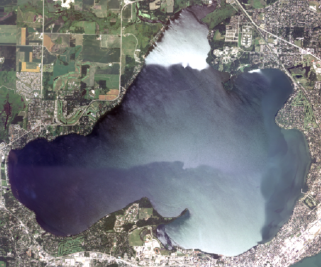
A square, staggered grid was chosen as the mesh for this study. It
was necessary to create a mesh of the site so I took a 2008 aerial image
and laid a grid over top of the image, consisting of squares 100 meters
X 100 meters. To cover the study area, it took 4000 squares, which
makes sense because the area of the lake is estimated at 40 km2.
Mesh grid of Lake Mendota Governing Equations Continuity
Equations of Motion
Equations were modified into a finite difference method using a Taylor Series Expansion and dropping off second order terms and higher. Finite Volume Element
All of this setup was then used to write a program using Matlab®. After >1000 lines of code, the program was running and I then used it to analyze a few simple cases for testing and then used it to analyze the water levels in the lake over a certain period of time and compared the results to the actual data at the dam. |

 (X-dir)
 (Y-dir)