| Calibration |
Calibration of the wave generation device was achieved via capacitance based wave gauges. |
| |
In order to verify the file read sample rate, free surface displacements were compared to the intended frequencies, and adjustments were made.
The computer clock running the LabView program showed a small deviation, yielding a sample rate of .0094s instead of .01s.
The adjustment to match sample rates was made in the sample rate output for the ASCII control file.
After adjustments were made, the system was verified to run at the intended sample rate in 5 consecutive trials |
| Signal Generation |
The servo motor controller is programed to recieve an analog voltage signal corresponding to velocity. |
| |
The motor controller must be set to scale the range of voltage to relate to the scale of incoming signals. Because of limitations due to the DAQ device used at the time of this experiment, only dc voltages in the range of 0-5v were supported. The controller was programmed to offset incoming voltage by 2500mv, which meant an incoming 2.5v signal would correspond to a zero velocity signal sent to the motor.
Because the device operated on velocity signals, files written as paddle displacement from the mean were transformed into velocity voltage using a finite slope method with the resolution of the output sample rate.
After a velocity file was written in ASCII format, the LabView program could then prompt the user and read the file and store its contents as a time dependant array. Working in conjunction with the DAQ device, the program would then output a single voltage to the wave maker, updating at every time step. |
| Wave Functions |
 |
| |
It was decided that the flume would be used at a mean depth of 10" (25.4cm) due to paddle size restrictions. With a set depth, we were restricted to a lower bound of wave frequencies that would behave as deep water waves.
For our trials, we attempted breaking waves with a variety of frequency bands, but the best results were from a range of 1.75Hz to 2.5Hz. With this frequency set, we divided the bandwidth into 32 frequencies. The dispersion equation (shown above) was solved for each frequency to obtain wave numbers (k). |
| |
 |
| |
By setting a breaking distance (xb) of 1.5m with respect to mean paddle position, and a breaking time (tb) of 10 seconds, we systematically solved the above equation for each wave number. This solution was achieved by setting displacement (x) to 0m and solving for t. The result would yield the point in time at which the paddle displacement would be 0 to produce the wave. This solution allowed for determination of phase shift (phi) of each function. (Wu 2006)
The resulting equations were unique in all variables (save tb and xb) and were superimposed to yield the displacement signal for the entire wave train. The sample interval (.0094s) was used to output a time-series ASCII file for wave generation. |
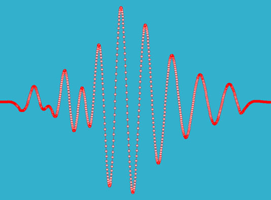
| Wave Signal: |
 |
| |
The resulting time series output was produced using a dispesion solver in matlab (Wu 2006) and was used as input into the LabView user-based motor conrol program.
Each node in the above graph represents a single sample of analog velocity sent to the servo motor. The motion acheived by the servo was scaled manually as to find the scale at which minimal energy was lost before breaking. |
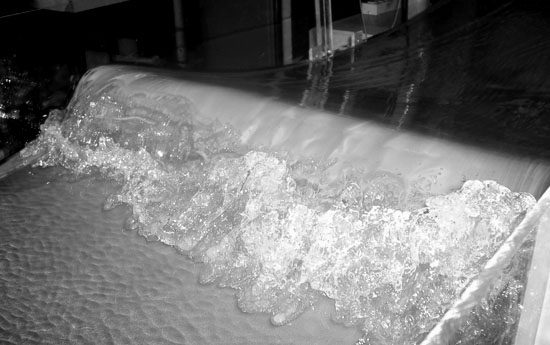
| Breaking Wave: |
 |
| |
Jordan Read (2006) |
