Introduction	Motivations &Objectives	Coastal Area	Results	Links

SWAN was developed at Delft University of Technology .  It is a numerical wave model that is used to estimate wave parameters.  It is based on the wave action balance equation.

where  are propagation velocities in the respective spaces.

? = relative frequency

? = wave direction

N = action density spectrum

The above equation takes into account the nonlinear transfer of energy from one frequency to another by wave-wave interaction, the transfer of wind energy to waves, energy dissipation due to bottom friction, depth-induced wave breaking, and energy dissipation due to whitecapping.

It is my understanding that as numerous other wave models, SWAN finds the solution to the above equation "in finite difference form throughout a grid placed over the coastal area where active wave generation is taking place.  As wave generation proceeds, the model computes the action density spectrum at each grid point and time step." (Sorensen, 177 & 178)

To Top of Page

2. Apply SWAN to Lake Mendota

SWAN can be downloaded at http://fluidmechanics.tudelft.nl/default.htm.  Chris Petykowski, a graduate student at the UW-Madison, was very helpful.  He downloaded and configured SWAN for me.  To apply SWAN to Lake Mendota I used four files.

1. application file.

2. batch file.

3. input file.

4 bottom file.

I could have also had files for boundary conditions, wave fields, initial conditions, and current fields.

An input file may look something like the following.

$*************HEADING****************************************
$
PROJ 'mendota 12-08-03' 'Z99'
$
$ PURPOSE OF TEST: Test of the wind generation on Lake Mendota
$
$ --|--------------------------------------------------------------|--
$ | This SWAN input file is for a test run of swan with wind |
$ | generation on Lake Mendota. Comp Grid = 100m x 100m |
$ --|--------------------------------------------------------------|--
$
$***********MODEL INPUT********************************** ***
$
SET NAUT
MODE STAT TWOD
$
CGRID REG 0. 0. 0. 9600. 8800. 96 88 CIRCLE 100 0.05 1.0 40
$
INPGRID BOTTOM REG 0. 0. 0. 479 439 20. 20.
READINP BOTTOM 1. 'mendota.bot' 3 0 FREE
$
WIND 18 337.5
$
$
INIT ZERO
$
GEN3 KOM 2.36E-05 3.02E-03 QUAD 2 0.25 3.0E07 5.5 6.7 -1.25 AGROW 0.0015
$
BRE CON 1.0 0.73
$
$************ OUTPUT REQUESTS *************************
$
CURVE 'CUA01' 4683. 7142. 70 6811. 520.
GROUP 'GRO01' 0 96 0 88
TAB 'CUA01' HEAD 'wnwinfo.tbl' HS DEP
PLOT 'GRO01' FILE 'Hs.PLT' ISO HS 0.05 0. 0.7
$
TEST 0,0
POOL
COMPUTE
STOP
$

The SWAN User Manual is a very useful resource.

The bottom file I used was simply the bathymetry of Lake Mendota which was prepared by Chris Petykowski.

After the four files listed above are prepared, they must all be placed in the same directory.  Then SWAN can be run in

MS-DOS.  An example of MS-DOS input is given below.
 
 

To Top of Page

3. View Results

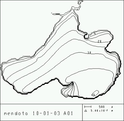
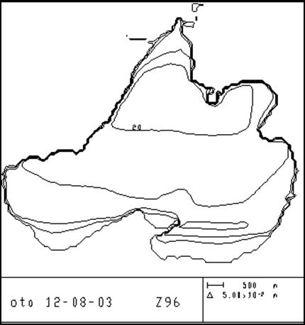
I viewed my SWAN results using View Companion 2000.  The following are a two examples.

Wind is from the South (180 degrees) 5 m/s.

the 20 contour is a Hs of .2m.

I compared the results from SWAN with hand calculations that I did using the SMB method.

4. Reference

Sorensen, RM (1997), Basic Coastal Engineering, 2nd Edition, Chapman & Hall
 
 

To Top of Page