Surface Water Modeling System (SMS) is a software to create
one-, two, and
three-dimensional hydrodynamic modeling. We used this software to plot
the bathymetry in our
study site. The
software can make bathymetry grid in rectangular/Square
grids and triangular grids. Triangular grid system was used to plot the
bathymetry to ensure better and more accurate coverage of the area.
Detailed
literature on the working of the software is available on line (http://www.ems-i.com/SMS/sms_8_1_new_features.html)
but the general procedure for making the grid is as follows:
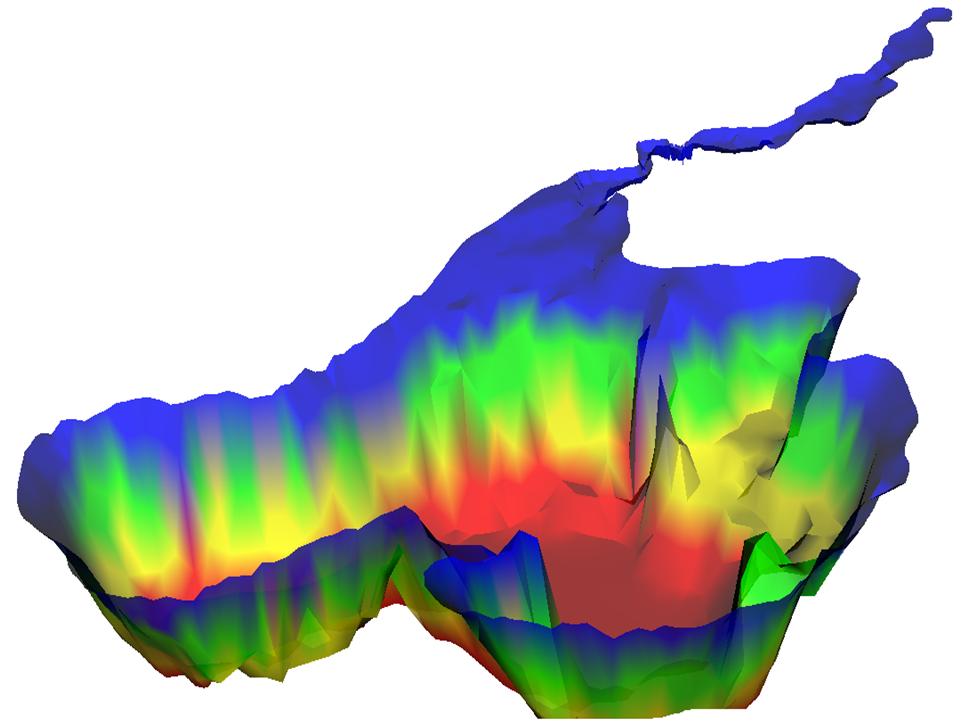
The
mesh/bathymetry map generated for our study site was as shown below(
the
vertical scale has been exaggerated 20 times for better assimilation
and the color represent certain depth ):
Figure 4: mesh/bathymetry depth
The area of our major focus was north of bridge at HW 113, which has the following bathymetry shape:
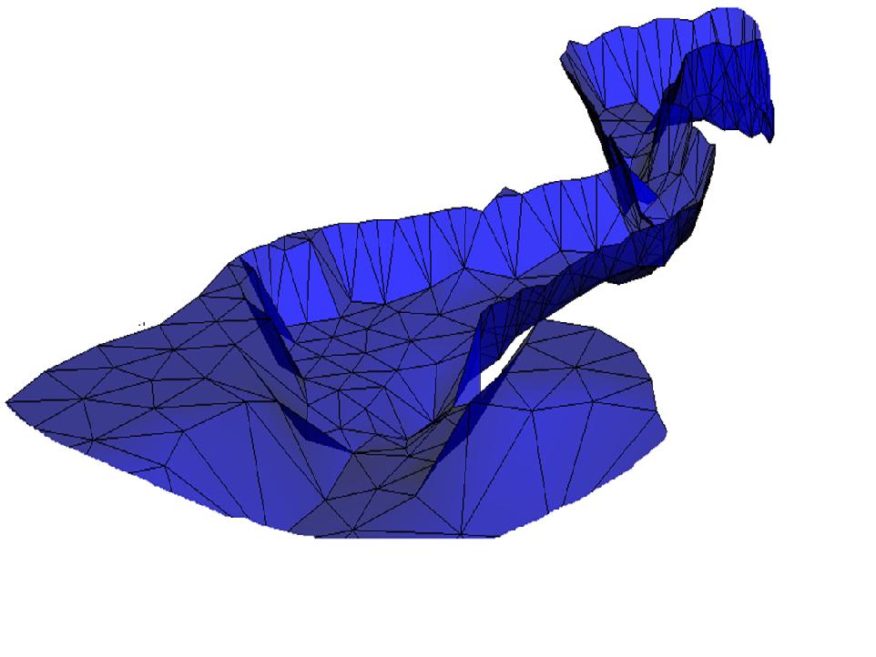
Figure 5: major focus area
Finite
Volume Coastal Ocean Model (FVCOM) was originally developed for the
estuarine
flooding/drying process in estuaries and the tidal-, buoyancy- and
wind-driven
circulation in the coastal region featured with complex irregular
geometry and
steep bottom topography.
FVCOM's
outputs are represented by
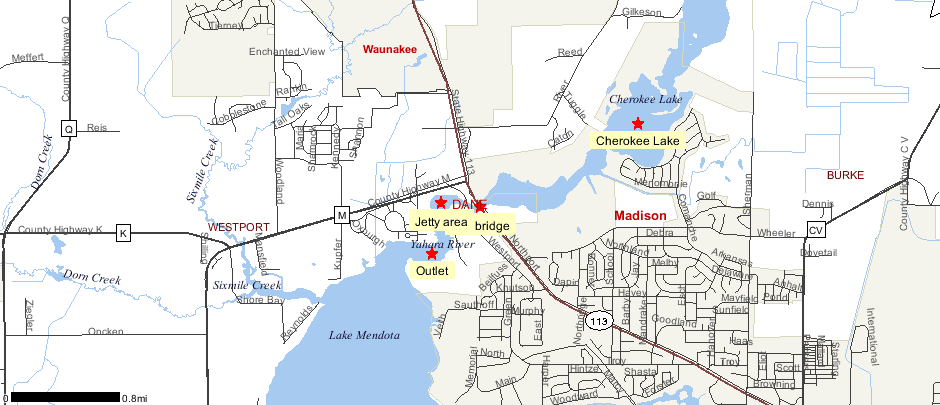
nodes. In order to narrow the details, we picked seven nodes (node 843 ,
node 921 , node 875, node 516, node 509, node 510 and node 639) as the representatives for
the wave calculation. These nodes are located at the outlet to Lake
Mendota,
the jetty area, the bridge and the Cherokee Lake.
Node 639, 510: Entrance to the
lake Mendota.
Node 509: Inside
the jetty areas.
Node 516: Near
the Bridges.
Node 843, 921, 875: Cherokee Lake.
Wind can strongly affect
the behavior of water waves (Especially,
the wave period (Ts) and wave height (Hs). In order to account wind into our calculation, we
downloaded the wind
information (for Madison area) of October from NOVVA. The average
daily wind speed (‘Ua’) and the wind direction (‘dir’) are listed in
table 1. The
average daily wind speed at 10 meters height is also listed in table
and it is calculated by Yao's emperical power law (appendix). The average wind
speed for
October , 2008 is 5.54 mph (2.47 m/s)
Table 1: wind infromation for 10/2008
| day | Ua(mph) | Ua(m/s) | U10(m/s) | Dir |
| 1 | 7.6 | 3.40 | 4.02 | SE |
| 2 | 2.8 | 1.25 | 1.48 | SE |
| 3 | 3.3 | 1.48 | 1.75 | SW |
| 4 | 1 | 0.45 | 0.53 | NW |
| 5 | 6.5 | 2.91 | 3.44 | NW |
| 6 | 10.3 | 4.60 | 5.45 | NW |
| 7 | 6.2 | 2.77 | 3.28 | NW |
| 8 | 4.9 | 2.19 | 2.59 | SE |
| 9 | 1.8 | 0.80 | 0.95 | SE |
| 10 | 5.2 | 2.32 | 2.75 | NW |
| 11 | 4.5 | 2.01 | 2.38 | N |
| 12 | 6 | 2.68 | 3.18 | N |
| 13 | 7.6 | 3.40 | 4.02 | NE |
| 14 | 2.1 | 0.94 | 1.11 | E |
| 15 | 3.4 | 1.52 | 1.80 | SE |
| 16 | 3.5 | 1.56 | 1.85 | SE |
| 17 | 0.8 | 0.36 | 0.42 | NE |
| 18 | 2 | 0.89 | 1.06 | NE |
| 19 | 10.8 | 4.83 | 5.72 | NE |
| 20 | 6.3 | 2.82 | 3.34 | SE |
| 21 | 3.3 | 1.48 | 1.75 | SW |
| 22 | 9.8 | 4.38 | 5.19 | NW |
| 23 | 11.2 | 5.01 | 5.93 | NW |
| 24 | 4.6 | 2.06 | 2.44 | NW |
| 25 | 6.6 | 2.95 | 3.49 | NE |
| 26 | 11.5 | 5.14 | 6.09 | SE |
| 27 | 9.9 | 4.43 | 5.24 | SE |
| 28 | 5.7 | 2.55 | 3.02 | SE |
| 29 | 2.2 | 0.98 | 1.16 | SE |
| 30 | 9.3 | 4.16 | 4.92 | NE |
| 31 | 0.9 | 0.40 | 0.48 | NE |
The fetchs from different wind blowing direction is also
estimated. The fetch for eight different direction is listed in
table 2
Table 2: Feth information
| Direction | Fetch,m |
| N | 368 |
| NE | 2656 |
| NW | 80.46 |
| S | 720 |
| SE | 80.46 |
| SW | 2656 |
| W | 176 |
| E | 192 |
| JONSWAP | ||||||
| U10(m/s) | F* | t* | Feff* | Limit | Hs*(m) | Tp*,(s) |
| 1.16 | 4692.703 | 15222.41 | 3291.11174 | duration limited | 0.091789 | 313.752652 |
| 4.92 | 8611.065 | 3589.024 | 376.774895 | duration limited | 0.031057 | 35.9192066 |
| 0.48 | 904700 | 36787.5 | 12364.2494 | duration limited | 0.177911 | 1178.72511 |
| Node | D, (m) | V,(m/s | L,(m) | d/L | T,(s) | H mean ,(m) | Hmax,(m) | Cg,(m/s) | E,(J) | P,(J/S) |
| 921 | 1.28 | 0.02 | 132.87 | s | 72.9 | 0.10098 | 0.181 | 0.020 | 3753.59 | 105.26 |
| 875 | 1.05 | 0.021 | 119.88 | s | 72.9 | 0.10104 | 0.181 | 0.021 | 3395.24 | 75.96 |
| 843 | 0.91 | 0.025 | 58.00 | s-IM | 72.9 | 0.10089 | 0.179 | 0.025 | 1624.00 | 43.94 |
| 516 | 1.18 | 0.028 | 66.37 | s-IM | 72.9 | 0.10068 | 0.178 | 0.027 | 1842.19 | 53.33 |
| 509 | 1.12 | 0.017 | 64.58 | s-IM | 72.9 | 0.10068 | 0.178 | 0.017 | 1792.86 | 47.79 |
| 510 | 1.09 | 0.018 | 63.70 | s-IM | 72.9 | 0.10066 | 0.178 | 0.018 | 1768.10 | 25.43 |
| 639 | 1.27 | 0.019 | 69.16 | s-IM | 72.9 | 0.10065 | 0.178 | 0.018 | 1914.37 | 48.20 |
note: s= shallow water, s-IM= shallow to interm