Abstract:

The goal of this exercise was evaluating two methods of tide prediction. The first method chosen was a form of Harmonic Analysis known as least squares method. The advantage to this method is that it allows the user to input known tidal frequencies in order to determine the amplitude of the specific constituent in question (i.e. K1, the Lunar Diurnal Constituent). These constituents allow for the classification of tides as well as aid in tide prediction. Boston Harbor six-minute tide data was used in this analysis. The second  method, also a form of Harmonic Analysis, was  a discrete Fourier Transform. The advantage with this method is that it allows the user to define the number of frequencies to be determined and outputs the specified amount. This type of analysis is quite useful in bodies of water that are not affected as much by gravitational forces, more high frequency waves. Two-minute tide data from Lake Mendota was used in this analysis.

Motivations and Objective:

As stated in the introduction, the goal of this project was to develop tools that could be used in tide prediction for ocean scale water bodies and also give some insight into what causes fundamental frequencies in smaller bodies of water in a  smaller setting. While all the equations have all been developed and put into practice, it was a chance to gain personal understanding of how the analysis is approached and some of the specifics with respect to the math involved in the derivation. The other personal objective was to get aquainted and comfortable with programming in MATLAB to gain some experience in data manipulation.
 

Coastal Environment of Targeted Area:

Boston Harbor has been the site of poor wastewater practices for over two hundred years. Waste was just dumped into the harbor and surrounding coastal area in the hope that the ocean would take care of the problem. This would turn out to be a false assumption and with rising tides, raw sewage would be brought directly to the harbor and its beaches making the environment uninhabitable for most of the habitat that the harbor once supported. This forced the people of Boston to examine the problems that their practices’ had caused, and scrambled to come up with a solution. One of the projects in progress presently include building a state of the art waste water treatment plant on Deer Island that not only removes most of the waste from the water, but distributes the effluent nine miles off the harbor coast to aid in the mixing and dilution process. The army corps of engineers along with the Massachusetts Port Authority has also undertaken a dredging project that is set up to allow boats more access to the tributary channels, at the same time cleaning out the contaminated sediment from the polluted water. Tide monitoring  will be an indicator of how these projects are affecting the harbor presently and the effects that could result in the future.

Contrasting Boston Harbor, Lake Mendota is self-contained and has less variable tides due to its relative size to that of an ocean. Like Boston, the lake has fallen victim to sewage effluent pollution which has in turn created  nutrient levels conducive to the expansion of large algal blooms. Dredging and filling have been implemented to make the land surrounding the lake more attractive to users of the area along with control structures that provide lower water levels in the fall and spring so as to minimize damage to infrastructure from the freeze-thaw process. These physical changes have all had an effect on the periods of the waves in the lake.
 

Approach to the Issues

The first step in any project like this is to get some background information so as to have some basis for getting started.  Professor Wu provided a paper that gave an explanation for the least squares method. It provided a general equation for N constituents (but in the case of the first part of this project, only N=4 were necessary). In order to gain a better understanding how the formulas worked, a general solution was obtained by hand for one and two constituents. In this specific application, the goal was to solve for 4 constituents including K1, O1, S2 and M2 based on their respective periods. These four were chosen as a means of calculating the form factor F. The form factor is a "rule of thumb" technique that allows for a quick characterization of types of tides: semi diurnal, mixed or diurnal.
 

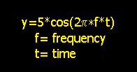
With some basic understanding the programming portion of the project began. After a slow start, the program was completed in a couple of hours and ready for actual data. Before that could occur however, the program required testing  to ensure the rather archaic style of programming actually yielded a valid result. This was achieved through creating a set of data that behaved according to the equation:

The test was conducted by running the data through the least squares program to see what the results yielded. Success would be realized if the amplitude of the K1 component output a value of 5 and the other three were zero (since the only frequency the data fit was that of the K1 component).

Once a duration of 2 months was found to have enough resolution in test data, the real Boston Harbor data was run through the program (6- minute data for two months from NOAA web site, site 8443970). With questionable results, the duration was increased to one year.  Since Boston is semi-diurnal, another check was added with the addition of three trials with one year data from a diurnal site in Corpus Christi, Texas (site 8775351).

Lake Mendota data was analyzed using a MATLAB code called Ncomponent (Wu, 2000). Using sections of two-minute data it calculated the dominant frequency of that data and plotted versus the amplitude at that frequency. This information was used to determine what was the dominant force driving the duration of the wave period and the corresponding frequency.

Results:

Discussion:
Results were positive for the first run, but did not yield exact numbers of one 5 and three 0's. The numbers were close and led me to believe that the program needed better resolution to produce better results. This introduced an opportunity to test the test data to try and find an optimum sampling frequency or duration of sampling to determine a threshold at which this technique will produce accurate results. Unfortunately the randomness of the data made results of the optimization testing less applicable, so it was decided after analyzing all of the  two month data for 1999, to increase the period to 1 year. Looking at even the one year data suggests that the duration will probably have to be increased to the decade scale to get any consistency in the results.

Another possibility to consider was the data itself. There is no better example of this than in the 1998 Texas data. The peak in the late summer months caused the form factor to increase in magnitude from the other two years in this study. This either suggests that a major storm occurred in late summer, or just a problem with the data logger over that period of time. Either way it is an anomaly that makes the results that were output by the program erroneous. This would suggest that one would have to closely examine all of the data before processing to eliminate the error associated with outliers.

The Mendota data fit the initial expectations. It is quite obvious that wind waves are a present based solely on visual inspection of the lake. They will not show up n these data however due to the fact that it at intervals of 2 minutes and the range of wind waves is in the order of seconds. The scale that this data falls onto is similar to that of a seiching motion. Seiching is  "the formation of standing waves in water body, due to wave formation and subsequent reflections from the ends." ref These basin oscillations cannot necessarily be seen with the naked eye, but the analysis of the data shows that the phenomenon does exist.

References:
The Fishery of the Yahara Lakes.  Wisconsin Department of Natural Resources., Technical Bulliten No. 181, 1992.

Emery,WJ and Thomson, RE, "Data Analysis Methods in Phyiscal Oceanography",Elsevier Science, 1998. (for Least squares reference).

R.M. Sorensen, Basic Coastal Engineering 2nd ed. Chapman & Hall, 1997

http://www.coastal.udel.edu/faculty/rad/seiche.html