Theoretical Levee Design for a Category 5 Hurricane in New Orleans

Alec Danielson

CEE 514

Introduction

Motivation

After watching the destruction of Hurricane Katrina on the news and listening to analysis about how New Orleans wasn’t prepared for a large hurricane, I wanted to design one of the levees that failed in New Orleans for a category 5 hurricane and see how much different it would be to the levee that was already in place. I wanted to see if my design was more robust, and I wanted to analyze some of the many aspects that go into designing a coastal structure.

Disclaimer

The analysis and design provided in this webpage are done using many simplified assumptions. There are too many conditions to consider that I do not have the expertise in to perform a complete analysis. I focused on the major design issues while still trying to account for the other potential issues.

Site Description

I chose to analyze the levees that failed near downtown New Orleans on Lake Pontchartrain. There were numerous failures along this section with many breaches over 30 meters in length. Lake Pontchartrain (Figure 1) is about 50 km across at its widest point and is approximately 5 meters deep for much of the lake. The bathymetry of the nearshore in Lake Pontchartrain (Figure 2) is spotted with dredging depressions. The lake bottom has been dredged numerous times for backfill on marginal coastal lands. The site rests on loose silt that was deposited by the Mississippi. This is the same silt that is currently being dumped into the Gulf of Mexico due to the shipping canals and controls. If more silt was allowed to deposit on the nearshore, the natural protection would be greatly increased and the need to design robust structures would diminish.

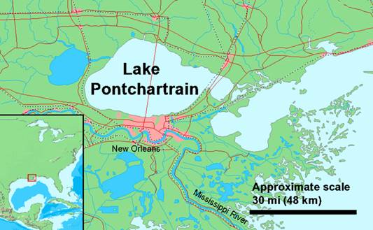
Figure 1 – Map of Lake Pontchartrain Arrow designates site location (Wikipedia 2005)

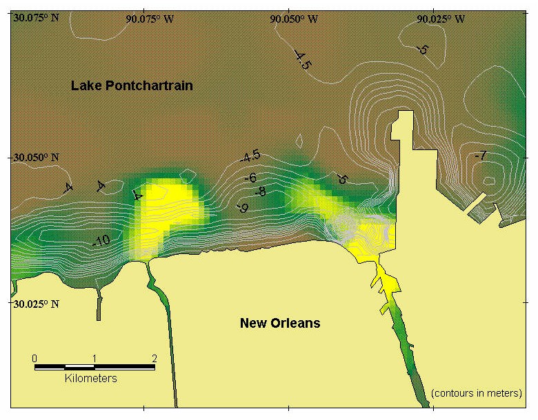
Figure 2 – Picture of near-shore bathymetry in Lake Pontchartrain The circular depressions represent the areas of dredging common near the shore of New Orleans. (United States Geological Survey, 2004)

Major Assumptions Made

I made numerous assumptions to simplify the problem including:

à Category 5 Hurricane (Wind Speeds 70m/s or 155 mph) See Saffir Simpson Scale below

à Storm lasted 6 hours (approximately the duration of a major storm for a single location)

à Fetch of 3200 meters (this was approximated using an east to west wind provided by a hurricane and the protection provided by land near the site location)

à Storm doesn’t weaken during the duration

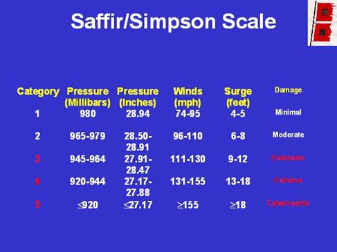
Figure 3 – Saffir Simpson Hurricane Scale Note that calculations were made using the lower limit of a Category 5 hurricane (155mph) (duedall.fit.edu)

Analysis

Storm Surge Calculation

Storm surge calculations were made using the closed basin analytical approach. The assumption of a straight-line wind was used over the distance of 3200 meters. Calculations were made along different depth segment to account for seafloor variability. Sample calculation is shown below.

∆d/∆x = Cd*U₁₀² / g*d

where ∆d = change in water depth from wind set-up

∆x = distance traveled

U₁₀ = Wind Speed

g = acceleration due to gravity

d = water depth

Cd = Drag Coefficient

where Cd = (1.21 + 2.25(1-5.6/U₁₀)²) x 10^-6

for U10 = 70m/s, d = 5m, ∆x = 32000m (rough approximation of problem)

∆d = 10m

Full segmented analysis was conducted on a spreadsheet with the following results

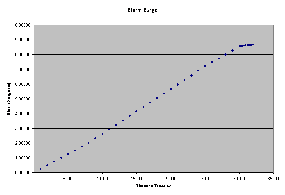
Figure 4 – Storm Surge Calculated for distance traveled Notice the linear increase in storm surge with depth until the near shore, where the dredging pits decrease the incremental storm surge

The total wind induced storm surge calculated was 8.7 meters (~28ft)

Wind Generated Waves

The JONSWAP method for calculating wind generated waves was used with the same assumptions (U = 70m/s, 6 hrs duration) used to calculate the storm surge. It was determined that the waves were fetch limited. Fetch limited means that the length of water over which wind can generate waves is limiting the development rather than the duration for which the wind has blown over the water. The complete analysis was performed in segments to see the change in wave height with the distance traveled. A sample calculation using the JONSWAP method is shown below.

1^st step – calculate F* F* = gF/U₁₀²

2^nd step – calculate t* t* = gt_d/U₁₀

3^rd step – calculate F*_eff F*_eff = (t*/68.8)^^1.5

4^th step – compare F* & F*eff if F* > F*eff ~ duration limited

if F* < F*eff ~ fetch limited

use smaller value for F**

5^th step – calculate Hs gHs/U₁₀² = 0.0016(F**)^^0.5

6^th step – calculate Tp gTp/U₁₀ = 0.286(F**)^^1/3

where F = fetch length

Hs = Significant Wave Height

Tp = Wave Period

t_d = duration

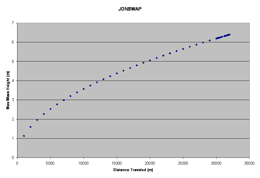
Figure 5 – Wave Height Calculations using the JONSWAP method Notice the slower increasing wave height with distance traveled indicating that the waves are becoming closer to fully developed

The wave heights calculated above using the JONSWAP method did not account for interaction with the lake bottom. The waves generated are very large and very long and Lake Pontchartrain is relatively shallow indicating that influence from the lake bottom will occur, and the condition of breaking waves might be present. From the relationship of conservation of power, I used the relationship between the dimensionless wave height and relative depth to determine the influence of the lake bottom (Figure 6). After accounting for the influence from the lake bottom, I combined the storm surge with the wave height data to determine a wave envelope progression. The wave envelope uses the storm surge level as the “mean” water level and then adds/subtracts the wave amplitude.

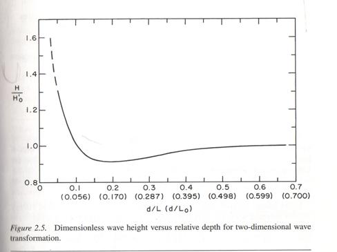
Figure 6 – Dimensionless wave height versus relative depth For shallow water conditions the wave height is limited to ~0.9Ho. Shallow water conditions exist for much of Lake Pontchartrain. (Sorensen, 1997)

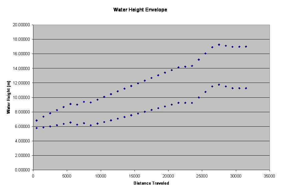
Figure 7 – Water Height Envelope Notice the increasing differences between the maximum and minimum wave heights with distance traveled.

Wave Run-up

With the incident storm surge and wave heights calculated the interaction with the levee must be considered. The design height of the levee depends not only on the storm surge and the wave heights, but also the wave run-up caused by the incident wave energy. Wave run-up is the dissipation of the wave energy after the wave breaks, and is a function of: deep water wave height and period, the surface slope, approaching depth, and roughness and permeability of the slope. Dimensionless analysis with a run-up factor of 0.5 (stone) was used for 3 different potential slopes. The permeability of a stone slope diminishes the run-up expected on a smooth impermeable slope by the factor of 0.5. The sensitivity of the wave run-up to slope angle can be seen by the calculations for the 3 different slopes. The slopes chosen were: 1.5H/1V, 2H/1V, and 2.5H/1V. These slopes are common slopes used in embankment design. The process for calculating wave run-up is described below.

Calculate Ho/gT²

with Ho/gT2 known use Figure 7 to determine wave run-up

Ho/gT² = 6.08/(9.81*8.15²) = 0.0093

from Figure 7 cot(1.5) R/Ho = 2 using the run-up factor of 0.5; R = Ho = 6.08

cot(2) R/Ho = 1.5 using the run-up factor of 0.5; R = 0.75Ho = 4.56

cot(2.5) R/Ho = 1.3 using the run-up factor of 0.5; R = 0.65Ho = 3.95

Figure 8 – Dimensionless run-up chart Run-up increases with increasing angle until the 1.5H/1V point. Any slope steeper than 1.5H/1V has less run-up and greater reflection

Wave run-up is the vertical distance from the average wave height. My calculated values gave a run-up that was equal to the wave height for the 1.5H/1V slope and run-ups that were smaller for the shallower slopes. The small values of run-up can be attributed to the permeability of the stone slope. Because the wave amplitude (H/2) and run-up are measured from the same datum, the larger of the 2 values is chosen for the design water level. With the storm surge, wave amplitude and run-up considered the design water level is:

∆d(tot) = ∆d(storm surge) + [∆d(wave amplitude) < ∆d(run-up)]

∆d(tot) = ∆d(storm surge) + ∆d(run-up) = 8.07 + 6.08 = 14.15m for 1.5H/1V

= 8.07 + 4.56 = 12.63m for 2H/1V

= 8.07 + 3.95 = 12.02m for 2.5H/1V

Design

The design was completed using similar designs as a blueprint and analyzing some of the site specific parameters. I selected a embankment earth dam as my preliminary design with varying slopes for the side walls. Shallower slopes have a shorter design height and should have more stable slopes while more inclined slopes would take up less land on the shoreline. I needed to select my materials before I completed any design.

Riprap Selection

The mass of the stones used for slope protection was determined using the Hudson Equation (see below)

M₅₀ = ρ_r H_10%³

Krr(ρ_r/ρ_w-1)³cotα

where M₅₀ = mean stone mass

H_10%= top 10% Wave Heights

ρ_r = density of rocks

ρ_w = density of water

Krr = riprap stability coefficient Breaking waves Krr = 2.2 Krr = 2.5 for nonbreaking waves

M₅₀ = (2550kg/m³*(6.08m)³) M₅₀ = 747 kg

2.2*(2550kg/m3/1000kg/m3-1)³*2.5

A limited range for the gradation of the riprap has been empirically determined:

where Wmax = 4.0W₅₀ -largest stones cannot weigh more than 4 times the average stone weight (determined above)

Wmin = 0.125W₅₀ -smallest stones cannot weigh less than 8 times the average stone weight

The diameter of the stone was then determined from the following relationship

Ds = 1.24(W_s/γ_s)³

Diameter of average stone was determined as

Ds = 1.24(( 747kg*9.81m/s2)/25kN/m3)^1/3 Ds = 0.824m

Similarly, the diameter of the smallest and largest stones were determined

Dmax = 1.308m

Dmin = 0.412m

Filter Selection

A filter layer is needed between riprap protection and sand fill to limit movement of the riprap and to prevent piping losses of the fill. The movement of riprap could occur, because of the extreme differences in size between the riprap and sand (the diameter of medium grained sand is ~0.2cm). Piping losses are when the movement of water forces particle movement in a earthen structure. The difference in size is once again the culprit for piping losses. An intermediate layer prevents the movement of the finer particles out of the structure. It has been empirically determined that the thickness of the filter layer should be twice the size of the diameter of the stone above. This equates to a filter layer thickness of 1.6m for my design.

The size of the filter is also determined empirically through the following relationship:

d₁₅(filter) < 4*d₈₅(layer below)

Assuming d₈₅ = 0.3cm

d₁₅(filter) < 1.2cm àthis places the filter in the gravel range

The backfill material was determined to be medium grained sand and the core was deemed to be a loam. Full material properties can be seen on Figure 7.

Bearing Capacity Analysis

With the general design of a core earthen embankment set, I tested the potential bearing capacity failure of the designs under the 3 different slopes. A bearing capacity failure could result in movement of the entire embankment. If a section of the embankment moved relative to the rest of the embankment, cracks could form and the levee would be in jeopardy. The potential for failure in this mode exists, because of the loose silt that is characteristic of New Orleans. The bearing capacity analysis was conducted using the STED program. The levee with slopes 1.5H/1V had the highest Factor of Safety (4.6) and is shown below (Figure 8)..

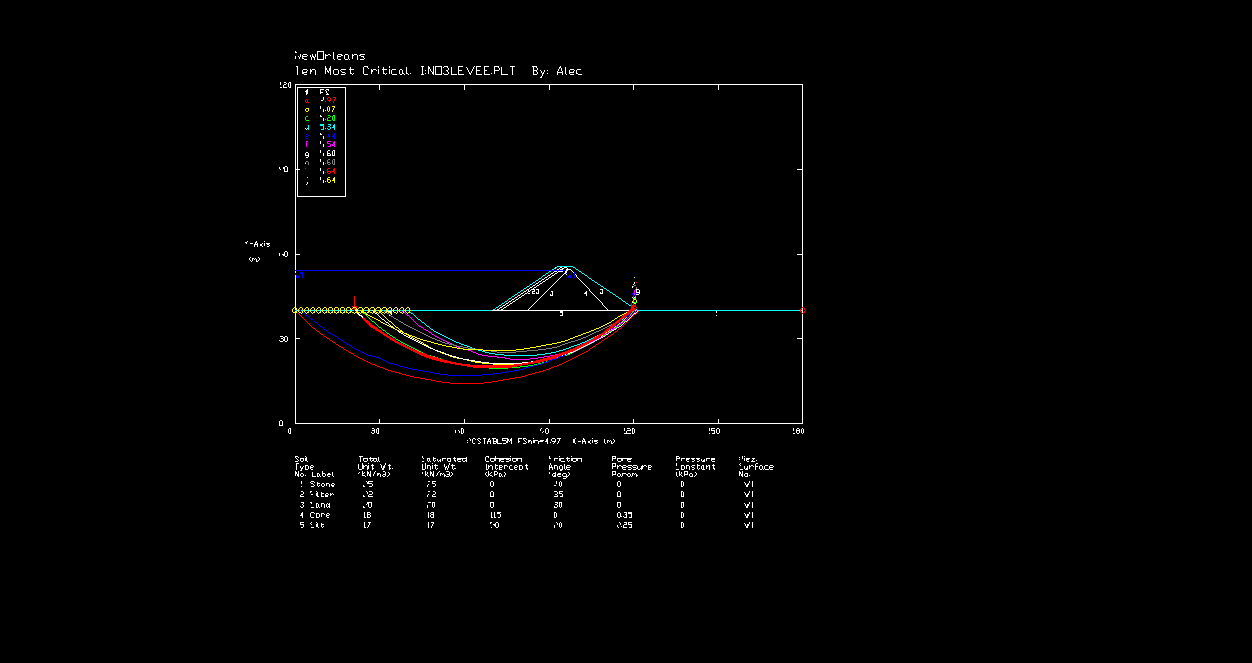
Figure 9 – Bearing capacity analysis Results of the bearing capacity analysis show that failure in this mode is unlikely with FS = 4.7

Slope Stability Analysis

The slope stability of the embankment was analyzed to determine if failure along any of the interface slopes would occur. The slope stability was determined using the Bishop Circular Method in STED. All of the embankment designs had very large factors of safety for the embankment slopes. Slopes of 1.5H/1V are manageable slopes for granular material (riprap, gravel, sand) and it was determined that pore pressure in the core resulting from the wave heights was not sufficient to cause failure along the interface of the core and sand fill.

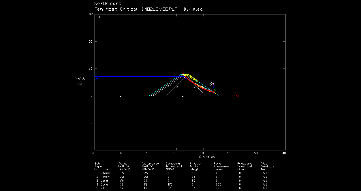
Figure 10 – Slope Stability analysis Slopes were deemed stable using the Bishop Circular Method

Seepage under the Embankment

I evaluated the seepage under the embankment using the principle of Darcy’s Law for flow through a porous media. I drew a flow net for the embankment under storm conditions. With the assumption of 0.5cm/s for the hydraulic conductivity of the silt under the dam I calculated the following seepage under the embankment.

Darcy’s Law Q = kiA

for a flownet Q/A = q =Nf/Nd*k

where q = specific discharge = flow per unit area

Nf = number of flow tubes = taken from the flow net = 6

Nd = number of head drops = head difference between the 2 sides of the embankment = 14.14 m

k = hydraulic conductivity = 0.5cm/s

q = 0.5 cm/s * (6/14) * 1m/100cm = 0.0024 m/s = 7.7 m/hr = 46 m/6hr storm

The seepage under the embankment is considerable. Foundation preparation in the form of a sheet pile or grouting would be necessitated for an effective design. For the calculated specific discharge, 46 cubic meters of water would pass under the embankment for every linear foot along the embankment. Seepage would greatly contribute to the flooding problem associated with large storms in New Orleans, with the nearshore inundated by seepage water. Uplift pressure underneath the embankment would also result because of the seepage, but was not considered. Earth embankments can more readily handle uplift pressures because the grains are able to move slightly to relieve some of the pressure. For a concrete design, the uplift pressures would be one of the controlling factors in the design.

Other Design Options

Several other options exist for levee design. A seawall can be built, with or without tiebacks, and a seawall can be used in combination with a levee. A seawall by itself would not be the preferred option for this purpose, because the seawall would have to be extremely high to meet the design wave height. New Orleans is very flat and is actually below sea level. There is not the natural near shore slope that could be used to apply support for a large seawall. The seawall/levee combination is a method that has been employed in New Orleans before. The major concern with the seawall/levee combination is the connection between them. If an earthen levee was used in combination with the seawall (Figure 10), potential for scouring at the interface would jeopardize the seawall portion of the structure. A seawall/levee combination could be constructed using concrete, and the structure could be designed to withstand the design wave heights proposed in this analysis, but the costs to build the structure would be even more astronomical than the earthen embankment design.

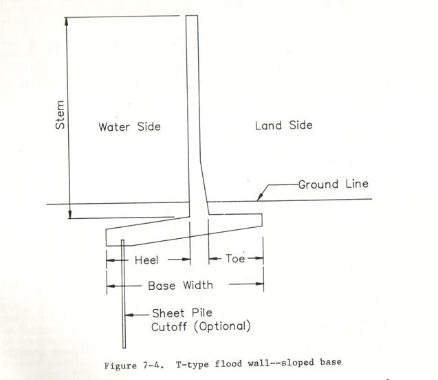
Figure 11 – T-type seawall that can be used with a levee or separately.

Selected Design

After analysis of the earthen embankment design and investigation of other design options, I chose the 1.5H/1V core earthen embankment design. All of the earthen embankment designs that I examined were very robust as would be expected for such an extreme design. The 1.5H/1V earthen embankment design was chosen, because it took less shoreline space, and would require fewer materials to build. This design is still very large and would require a large quantity of earth materials. The loam used to make the core would be compacted 5% wet of optimum. This is a value that has proven to be effective in numerous designs. The selection of sand for the backfill is not critical and would be taken from the nearest source. Riprap and gravel used for slope protection and the filter would be selected from the nearest source that meets the predetermined design requirements.

Comparison to Actual Levees

The levees in New Orleans during Hurricane Katrina were much shorter than the theoretical levee that I am proposing. The US Army Corps or Engineers designed the levees to withstand a Category 3 hurricane. The levees in New Orleans were primarily concrete embankments with seawalls on top. The levee heights for the section of New Orleans used in this analysis is given in Figure 12.

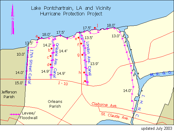
Figure 12 – Levee heights along Lake Pontchartrain in New Orleans.

To check my analysis of water level fluctuations I chose to recalculate my design wave height for a category 3 hurricane and compare my design height to that of the USACE’s. The storm surge calculated using the same method was 4.3m, with an additional wave height of 2.3m. My theoretical design water level for a category 3 hurricane is therefore 6.6m or ~21ft. Using my methods I calculated a design height that was about 1m higher than the USACE’s. The design completed by the USACE is much more in depth and complete, but I validated my approximation of a theoretical levee design for a category 5 hurricane in New Orleans.

Sources

J.R. Compton and S.J. Johnson, "Earth and Rock-Fill Dams General Design and Construction Considerations," Department of the Army Corps of Engineers., Washington, D.C. 20314, Tech. Rep. EM 1110-2-2300, 1971, 1971.

A.L. Goldin and L.N. Rasskazov, Design of Earth Dams, Brookfield, VT 05036: A.A. Balkema, 1992.

R.M. Sorensen, Basic Coastal Engineering, 115 Fifth Avenue New York, NY 10003: Chapman & Hall, 1997.

US Army Corps of Engineers, "Retaining and Flood Walls," Army Corps of Engineers., Washington, D.C. 20314, Tech. Rep. EM 1110-2-2502, 1989, 1989.

Coastal Engineering Manual, Army Corps of Engineering

Chin Wu, Phd University of Wisconsin-Madison