Storm Tracking on Lake Superior
Introduction
A large storm was predicted to hit the shores of Bayfield County from
Saturday, November 22nd, through Monday, November 24th. Mike Swenson, a
graduate student in the Department of Geological Engineering, and I, an
undergraduate in the Department of Geological Engineering, traveled up to
Bayfield County early Saturday morning to record the effects of this storm.
According to the
NOAA website, we were expecting winds to reach over thirty
miles per hour, producing wave heights up to fourteen feet. The storm was
not quite as strong as expected, but the following describes what we
encountered. After the storm we traveled back to Madison to analyze our
data. My goal was to measure the wave run-up, and to compare these
observed values to the run-up predicted using the Hunt (1959) and Wilson (1989)
methods.
Collecting Data
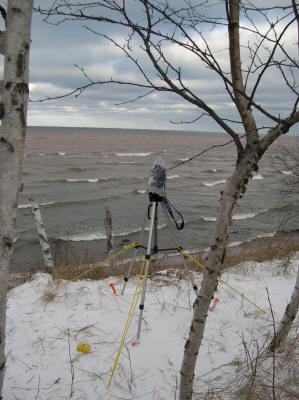
The picture to the right shows the camera setup on the top of the bluff at
the N-6 site. The camera needed to be secured to prohibit it from tipping over
from the force of the winds. The orange stakes at the base of the legs of the
tripod were set so when we came back we could mount the camera in the same exact
location. This would've worked, having also taken into account the angle of the
camera, the length of each leg of the tripod, and the zoom on the camera.
Apparently, the camera we used on November 23rd had a narrower view than the
camera used on the 24th, even though both cameras were fully zoomed out. This
caused some discrepancies in correlating the run-up for the two days.Two
recordings at the N-6 site were taken, one during the storm conditions, on
November 23rd, and the second (shown here) on November 24th, during intermediate
conditions. Each recording lasted one hour. During the storm
conditions, we were forced to endure the bitter winter storm. Snow was
blowing in from the lake, and would build up on the protective case on the
camera. This meant that during that hour, one of use would need to standby
and wipe the focal area clean every few minutes. We tried applying Rain-X
to the focal area, but this didn't work all that well.
While the camera was filming, and Mike was wiping the lens, I was assembling
a measuring stick that would be used to provide a scale to measure the distance
the wave traveled up shore. This turned out to be quite a process,
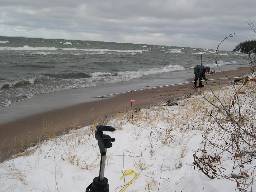 because
the markings on the measuring stick were not large enough to see from the top of
the bluff. We used duct tape to signify five foot increments, and
electrical tape to signify one foot increments. These both proved hard to
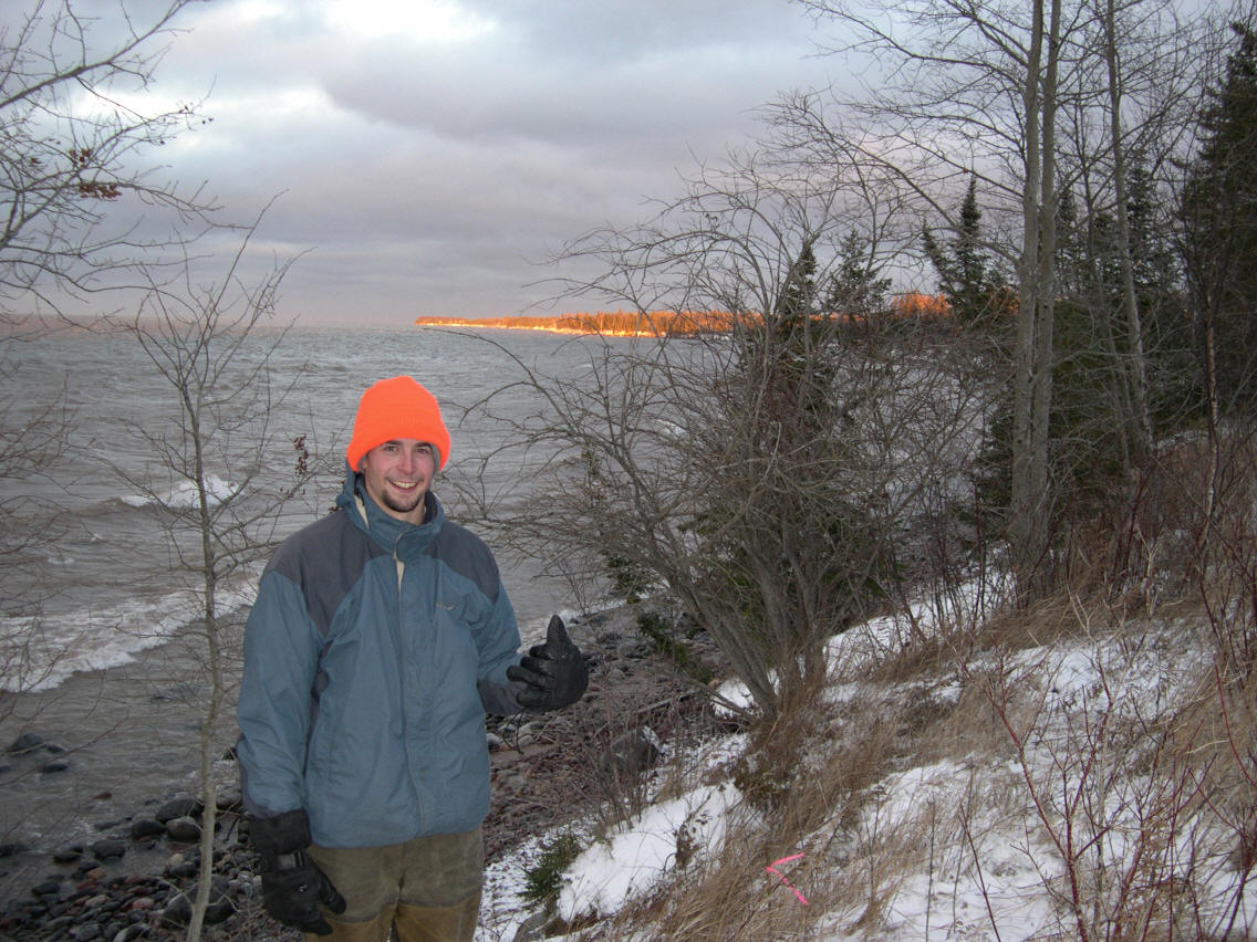
read, but were manageable. To the left is a picture of me and the
measuring stick at a different site. We used another, similar method, to
compare with the first method. We took a five foot section of the
measuring stick and taped it off at one foot increments. These tapings
were easier to read, but here errors could have occurred when the stick was
flipped end-for-end from the toe to just in front of the mean water level.
because
the markings on the measuring stick were not large enough to see from the top of
the bluff. We used duct tape to signify five foot increments, and
electrical tape to signify one foot increments. These both proved hard to
read, but were manageable. To the left is a picture of me and the
measuring stick at a different site. We used another, similar method, to
compare with the first method. We took a five foot section of the
measuring stick and taped it off at one foot increments. These tapings
were easier to read, but here errors could have occurred when the stick was
flipped end-for-end from the toe to just in front of the mean water level.
One last thing we measured at the site was the beach slope. This was
done using an inclinometer.
Data AnalysisTo analyze the videos,
a scale was needed to measure the distance each wave traveled. This was
done by taking a piece of Saran Wrap, and taping it over a television screen.
The video segments when the measuring stick was used were viewed, and the scale
on the stick was transferred to the Saran Wrap with a marker. This
provided a scale for all the waves recorded. The distance the waves
traveled up shore were recorded every other ten minutes of each one-hour storm.
This provided a good estimate of the wave action during that hour.
The distance the waves traveled were plotted over over the one-hour
duration in which they took place. Knowing the beach slope, α, these
distances were then converted to run-up, which is the vertical distance traveled
from the mean water level, and is shown below.
Where: Run-up = sin(α)*distance recorded

These were plotted during over the over a one hour interval as well, and can
be seen below.
Predicting Run-up
1) Determining Significant Wave Height using
JONSWAP method
In order to determine the predicted run-up, the significant wave height
is needed. Given the fetch (the distance the wind travels across the
water), F, the wind speed, U10, and the duration of the wind, td,
the significant wave height can be calculated using the JONSWAP (Joint North Sea
Wave Project) method.
The first step is to determine if the storm is fetch limited or duration
limited. To do this, F* and Feff* need to
be calculated.
1) F* = gF/(U102)
where g = gravitational acceleration (32.2 ft/s)
and
2) Feff* = (t*/68.8)1.5 where t*=
gtd/U10
If F* < Feff*, then the
storm is fetch limited. If F* > Feff*,
then the storm is duration limited.
The significant wave height, Hs, for a fetch limited storm is:
3) Hs = ((U10)2(0.0016)(F*)0.5)/g
The significant wave height, Hs, for a duration limited storm is:
4) Hs = ((U10)2(0.0016)(Feff*)0.5)/g
2) Classifying
Wave-Break
Knowing the significant wave height, the surf similarity parameter,
ξo, can be calculated to determine the
breaker classification.
5) ξo= (tan
α)/((Hs/(Lo)0.5) where α is the slope of the beach, and Lo is the deepwater
wavelength.
Lo = 1.56T2
where T is the wave period, determined by how much time it takes for one wave
to pass a given point, this value is recorded in meters, and needs to be
converted.
The wave is a spilling breaker if: ξo
< 0.5
The wave is a plunging breaker if:
0.5 < ξo < 3.3
The wave is a surging breaker if: ξo
> 3.3
3) Determining Run-up using Hunt (1959)
and Walton (1989)
method
Knowing the significant wave height, run-up, R, can now be determined.
If 0.1 < ξo < 2.3
6) R = Hs*(tan
α)/(Hs/Lo)0.5
If ξo is large, then
7) R = Hs*(sin
α)/(Hs/Lo)0.5
Predicted
Results1)
Storm Conditions
During the storm, the winds were out of the
northeast, blowing 30 miles per hour. The fetch length determined was 250
miles, disregarding the effects of Isle Royale. The winds were blowing in
this direction at varying speeds for over 24 hours. U10 was
chosen to be 20 miles per hour based on the variance of wind speed. The
time duration was chosen to be 24 hours, based on the data attained from the
national weather service.
Given this,
the storm was classified as duration limited, and the significant wave height,
Hs, was found to be 9.67 feet.
Given the amount of waves that hit the shore
during the hour, the period, T, was found to be 7 seconds. This correlated
to a deep-water wavelength of 250 feet. Knowing the slope of the beach was
6.5 degrees, the surf similarity parameter was found to be 0.579. These
waves are classified as plunging.
Plugging the values for wavelength, Lo,
slope,
α, and significant wave height, Hs,
into equation (7), the predicted run-up value could now be obtained.
Predicted run-up, R, for the storm conditions was found to be 5.6 feet.
2) Intermediate Conditions
The next day, November 24th, the winds had quieted, and shifted direction.
They were now blowing out of the northwest at 18 miles per hour. The fetch
length determined was 25 miles, and the duration of the northwest wind was 15
hours based on data obtained from the
national weather service.
Given this, the winds were again classified as
duration limited, and the significant wave height, Hs, was found to be 3.59
feet.
Given the amount of waves that hit the shore during the hour, the
period, T, was found to be 4 seconds. This correlated to a deep-water
wavelength of 80 feet. Knowing the slope of the beach was 6.5 degrees, the
surf similarity parameter was found to be 0.538. These waves are
classified as plunging.
Plugging the values for wavelength, Lo, slope,
α, and significant wave height, Hs,
into equation (7), the predicted run-up value could now be obtained.
Predicted run-up, R, for the intermediate conditions was found to be
1.9 feet.
Comparing
Predicted Values to Observed Values
Storm Predicted
Storm observed
Run-up: 5.6 ft
Average Run-up: 3.3 ft
The predicted run-up for the storm conditions was 2.3 feet greater than the
observed run-up. This may have been due to the predicted significant wave
height. The significant wave height was 9.67 feet, and may have marked the
upper limit of the waves recorded during the storm. From the videos, and
observing the waves first hand, the largest waves may have reached heights close
to ten feet, but many of them were much smaller. The average wave height
were probably much closer to six or seven feet.
Intermediate Predicted
Intermediate Observed
Run-up: 1.9 ft
Average Run-up: 2.0 ft
The predicted run-up for the intermediate conditions was very close to the
observed run-up. This leads one to believe that the prediction tools
described above can provide accurate results. The predicted significant
wave height value, 3.59 feet, seems to be much closer to what was actually
observed at the site.
Possible Causes
for ErrorsErrors may have occurred in several areas, but
surprisingly enough, the predicted values did not fall far from the observed
values. Errors in our measuring equipment may have affected our results,
because the measuring stick was hard to read, especially during the storm
conditions. The predicted margin of error of our measurements fell within
one to two feet. Another inaccuracy may have been do to the fact that we
used two different cameras for the different conditions. They were set up
exactly the same, but when both were fully zoomed out, the camera that recorded
the intermediate conditions had a wider view. This was accounted for, by
measuring the beach on both days.
Another possible cause for error was the
assumption of the location of the mean water table. This was assumed to be
at 43 feet from the the toe of the bluff, based on still water conditions during
the summer of 2003. The effects of set-up due to wind-induced shear
stress, the Coriolis effect, atmospheric horizontal pressure gradients, wind
wave setup, long wave generation caused by moving pressure disturbance, and
precipitation and runoff were disregarded. The effects of refraction due
to the northeast winds traveling past the Keweenaw Peninsula were also
disregarded.
The largest source of errors, however, were most likely due to
the fetch distances and time durations used in the predicted calculations.
The winds were not as regular as the equations are lead to believe, and this may
have been the cause for the larger predicted significant wave height during the
storm conditions.
Storm Tracking on
Lake Superior, 2003 - Hans Hoffman
This project was done during my last semester at the University of Wisconsin
- Madison. I graduated in December with degrees in Geological Engineering
and Geology. I did this project for Coastal Engineering 514 which is instructed
by Professor Chin Wu. The blaze orange hat was used to keep from getting
shot during deer season, and the sun in the background was the only sun we saw
the whole time we were up on Lake Superior.